润滑科技信息平台

润滑百科的目标：分享全球各地的知识，创建一个任何人都可以访问的百科全书。每个人都可以阅读、撰写、编辑和分享。如果您想投稿或有任何建议，请通过电子邮件、微信、QQ及电话联系我们!具体联系方式详见本网页右侧！

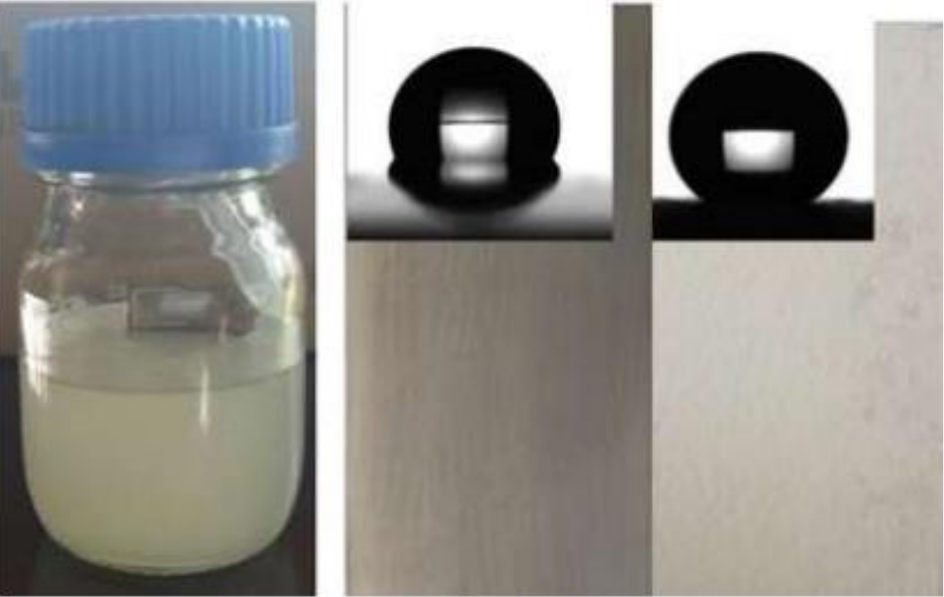
Area of contact between moving surfaces – Bowden and Tabor Home Wiki Area of contact between moving surfaces – Bowden and Tabor Area of contact between moving surfaces – Bowden and Tabor Manoj Rajankunte Mahadeshwara March, 4 2025 Table of Contents Introduction Experimental modifications Important findings Conclusions Reference Introduction When two plane surfaces are brought together, the area of intimate contact is much smaller than the apparent area. Even if the surfaces are carefully polished and made as flat as possible, they will still have hills and valleys at the microscopic level. The upper surface will rest on these irregularities, creating large gaps between other areas that are significantly larger than the dimensions of a molecule. The exact size of these irregularities and the degree of flatness of the surfaces are not well understood. This further changes with surfaces in contact under stationary and moving conditions. It is important to study how the area of contact changes within these moving surfaces in contact by understanding their electrical properties. Bowden and Tabors experiments have given greater insights into this field. Experimental modifications Previous methodology: Two crossed cylinders were arranged with their axes at right angles. Electrical conductance (A) was measured using a current-potential method. A known current (i) was passed through the contact, and the potential difference (v) was measured using a high-resistance potentiometer or galvanometer. The conductance was calculated as A=i/v. The load on the contact surfaces was varied by: Using water or mercury to adjust the weight (load range: 20 g to 6000 g). Applying larger loads (up to 1000 kg) with a lever machine and a spring balance. The contact surfaces were prepared through fine grinding, polishing, chemical etching, or scraping. Although surface preparation had minimal impact on results, scraping improved reproducibility. The measurements were extended to moving surfaces, with a method like the previous one, but with the potentiometer replaced by a rapid-response instrument like an Einthoven galvanometer or a cathode-ray oscillograph. Friction was measured using a high-frequency apparatus like that described in the previous paper. The lower surface, in the form of a flat plate, was driven at a constant rate by a water piston. The upper surface, which rested on it, was typically curved. Both the conductance and friction measurements were recorded simultaneously using the same moving-film camera, ensuring a synchronized record of both quantities. Important findings These experiments clearly demonstrate that the contact area between moving surfaces does not remain constant. While the average value of the conductance is similar to that observed with stationary surfaces, significant fluctuations can occur during sliding. These fluctuations are closely correlated with frictional stick-slip behavior, and the exact nature of these changes depends on the type of metals involved. In the case of a curved slider made of high-melting metal sliding on a low-melting metal, the area of intimate contact increases during the stick phase. However, when slip occurs, there is a sudden decrease in this area. These results strongly support the earlier suggestion that friction under these conditions is primarily caused by small irregularities on the high-melting metal ploughing through the surface of the softer metal. The characteristic “cut scratch” is observed with this behavior. In the case of a low-melting metal sliding on a high-melting-point metal, the behavior is the opposite of that observed with the high-melting metal on low-melting metal. The conductance decreases during the stick phase. However, once slip occurs, the conductance rises to a maximum value. This supports the suggestion that the local high pressure combined with the temperature rise from frictional heat causes the lower-melting metal to weld or solder onto the surface of the higher-melting metal. As a result, the area of contact is maximized. During the stick phase, the increasing pull causes these soldered junctions to become thinner (decreasing conductance) until they suddenly break, leading to slip. This process then repeats itself. When both surfaces are made of the same metal, conductance measurements show that the area of contact is somewhat greater and remains much more constant during sliding. During sliding, only small variations in this conductance occur. The friction is high, exhibiting slow fluctuations, and the characteristic torn track is formed. This behavior is generally observed with similar metals, as long as they are homogenous. These conductance measurements support the suggestion that in the case of similar metals, mutual welding of the two surfaces takes place. The local high pressures and temperatures cause both surfaces to flow, contributing equally to the formation of welded junctions. These mutual junctions are likely easier to form, resulting in a greater real area of contact and increased friction. When movement occurs, both surfaces are damaged, and the metal in the resulting track becomes severely distorted and torn. Conclusions Measurements with moving surfaces reveal that the area of contact fluctuates rapidly during sliding. These fluctuations are closely correlated with changes in friction and temperature, indicating intermittent clutching and breaking away of the surfaces, with metallic junctions being formed and broken. The nature of these junctions depends on the physical properties of the metals involved. Even when the metals are lubricated with mineral oils or other lubricants, metallic contact can still occur through the lubricant film. Fluctuations in the area of contact are observed during sliding, and the behavior may be similar to that of unlubricated surfaces. Reference [1] Bowden, F.P. and Tabor, D., 1939. The area of contact between stationary and moving surfaces. Proceedings of the Royal Society of London. Series A. Mathematical and Physical Sciences, 169(938), pp.391-413. ; Manoj Rajankunte Mahadeshwara I am a postgraduate researcher at the University of Leeds. I have completed my master's degree in the Erasmus Tribos program at the University of Leeds, University of Ljubljana, and University of Coimbra and my bachelor's degree in Mechanical Engineering from VTU in NMIT, India. I am an editor and social networking manager at TriboNet. I have a YouTube channel called Tribo Geek where I upload videos on travel, research life, and topics for master's and PhD students. -->

Area of contact between stationary surfaces – Bowden and Tabor Home Wiki Area of contact between stationary surfaces – Bowden and Tabor Area of contact between stationary surfaces – Bowden and Tabor Manoj Rajankunte Mahadeshwara February, 25 2025 Table of Contents Introduction The modified derivation Experimental Setup by Bowden and Tabor Important Results and discussion Conclusion Reference Introduction Hertz’s 1881 work established theoretical equations describing elastic deformation and the contact area between curved surfaces under load. Subsequent researchers, like Bidwell and Meyer, investigated electrical conductance in contacting materials, with Meyer linking contact resistance to pressure, though later studies suggested surface contamination affected his results. Later Binder (1912) demonstrated that conductance was smaller than expected, proposing that actual contact occurred over a small fraction of the surface. Experimental verification followed, with varying interpretations, such as Pedersen’s idea of a high-resistance transitional layer. Finally, Holm’s extensive research from 1922 onwards showed that contact resistance for clean metals adheres to Ohm’s Law and arises from “spreading resistance” due to current constriction in small contact areas. He concluded that flat surfaces consist of numerous small contact points. The modified derivation When a metal is very soft and subjected to high pressure, the contact area can approach the size of the entire metal surface. In such cases, the spreading resistance decreases, and according to the conditions where the radius of the contact area (a) equals the radius of the metal surface (r), the spreading resistance becomes zero. Hence the modified equation for electrical conductance (Λ) can be written as. Λ = 2λ (a*r/(r-a)) Experimental Setup by Bowden and Tabor Two crossed cylinders were arranged with their axes at right angles. Electrical conductance (A) was measured using a current-potential method. A known current (i) was passed through the contact, and the potential difference (v) was measured using a high-resistance potentiometer or galvanometer. The conductance was calculated as A=i/v. The load on the contact surfaces was varied by: Using water or mercury to adjust the weight (load range: 20 g to 6000 g). Applying larger loads (up to 1000 kg) with a lever machine and a spring balance. The contact surfaces were prepared through fine grinding, polishing, chemical etching, or scraping. Although surface preparation had minimal impact on results, scraping improved reproducibility. Figure-1 Figure of the cylinder arrangement [1] Important Results and discussion The measured conductance values between metal surfaces are similar to the specific conductivities of the metals, indicating that the resistance observed is mainly metallic (or carbon/carbon) and not due to oxides or surface contaminant films. It would be highly unlikely for the electrical conductivities of oxides or other films to match the metals’ conductivity order. If contaminating films are present, they must be very thin, contributing minimally to the electrical resistance. The results clearly show that conductance varies in an orderly fashion with the applied load. If elastic deformation occurs at the contact, the conductance should be proportional to the cube root of the load. However, if plastic flow occurs, the conductance would be proportional to the square root of the load. Due to uncertainties in the conductance measurements, distinguishing between these two behaviors can be difficult. For surfaces that make contact in a single region (e.g., crossed cylinders or sphere-on-flat), the measured conductance values suggest that intimate contact occurs across the entire deformed area. Despite the radius of curvature of the spherical surface varying by a factor of at least ten, the conductance values and the slope of the curves are almost identical. This suggests that, as long as the contact is localized in a single continuous area, the conductance—and therefore the real contact area—remains largely unaffected by the shape and radius of curvature of the surfaces. It is observed that, despite the potential contact area being vastly larger for the flat surface compared to the curved surface, the measured conductance is of the same order of magnitude. However, experiments show that the actual conductance is only about twice as large. This indicates that only a small fraction of the flat surface is in intimate contact, with contact occurring at several “legs” or “bridges.” It is also noted that the conductance for both sets of flat surfaces is nearly the same, even though their apparent areas differ by a factor of 30. This leads to the conclusion that the conductance is largely independent of the apparent surface area and is primarily influenced by the applied load. In the case of flat contacts, it is challenging to precisely estimate the real contact area based solely on conductance measurements. The conductance depends on both the size and the number of metallic bridges. Since the spreading resistance of each bridge is inversely proportional to its diameter, and the contact area is proportional to the square of the diameter, it follows that for a given conductance, the contact area is inversely proportional to the number of bridges. While the exact number of bridges is uncertain, it is clear that for flat surfaces, the number of contact points cannot be fewer than three. Conclusion It is clear that for flat surfaces, the real contact area, even under significant loads, is only a small fraction of the apparent area. The flat surfaces are kept apart by small surface irregularities that create metallic bridges. Under applied pressure, these bridges either flow or their number increases until their total cross-section is large enough to support the applied load. In general, the load-conductance curve for flat contacts appears to be steeper than for curved surfaces. However, it is challenging to propose a satisfactory quantitative hypothesis to fully explain this behavior. Reference [1] Bowden, F.P. and Tabor, D., 1939. The area of contact between stationary and moving surfaces. Proceedings of the Royal Society of London. Series A. Mathematical and Physical Sciences, 169(938), pp.391-413. ; Manoj Rajankunte Mahadeshwara I am a postgraduate researcher at the University of Leeds. I have completed my master's degree in the Erasmus Tribos program at the University of Leeds, University of Ljubljana, and University of Coimbra and my bachelor's degree in Mechanical Engineering from VTU in NMIT, India. I am an editor and social networking manager at TriboNet. I have a YouTube channel called Tribo Geek where I upload videos on travel, research life, and topics for master's and PhD students. -->

Adhesive Wear Modelling Methods Home Wiki Adhesive Wear Modelling Methods Adhesive Wear Modelling Methods TriboNet January, 28 2025 Table of Contents Introduction Wear Models Phenomenological approach Asperity Level Approach Rough surface Smooth surface Surface References Introduction Wear in dynamic systems significantly impacts performance, efficiency, operational costs, and safety. Predicting wear using computer simulations, empirical data, or theoretical frameworks is crucial for determining system reliability and durability. Haibo et al. [1] Reviewed wear modelling methods and depicted that wear modelling could be on macro, micro, or atomic scales. In light of this, wear modelling could be divided into a phenomenological approach or real contact conditions; the former utilizes physical understanding and experimental observation, i.e., macroscale level. In phenomenological technique, assumptions must be made, and empirical coefficients must be determined. Those models are constrained by their assumptions and lack generality, even though they provide accurate predictions for a specific range of operations and rely on the constraints of the empirical coefficients. Archard’s theory [2] and Rabinowicz’s criterion [3] These are examples of such models. The second method, such as asperities contact models, implements advanced numerical techniques to find the wear at micro- or atomic levels under relaxed assumptions and more realistic conditions; however, analytical models have been utilized for material and fracture estimation, and the actual surface characteristics may need to produce specific and accurate results. In the next section, microscale modelling techniques have been introduced. Wear Models Phenomenological approach An example of this approach is Archard’s wear model which is a famous model to evaluate adhesive wear. Theoretically, the Archard wear model estimates the adhesive wear volume of softer material. The model is named after Archard publicizes his work [2]; He said that the wear volume depends on the normal load and sliding distance and is inversely proportional to the hardness of the softer material. The wear volume (W) is defined as [4]: W = (K*P*S)/H – Equation-1 Where P is the normal force, S is the sliding distance, H is the softer material hardness, and is the dimensionless wear coefficient, and commonly used is the dimensional wear coefficient which is found experimentally and its value depending on lubricity condition and wear severity 1e-2 to 1e-9 [4] depending on the type of surface and lubricity condition. It’s commonly explained the wear rate is wearing volume per sliding distance (w) which is defined by [4]: w = (K * P) – Equation-2 Asperity Level Approach Asperity-level models for wear prediction offer valuable insights into wear phenomena, allowing for the estimation of wear volume and particle morphology. A prominent model developed by A. Greenwood and J. Williamson (GW model) [5], describes contact between rough, deformable surfaces, assuming that each asperity is loaded independently as shown in Figure 1. In this model, all asperities are hemispherical, with a constant radius of curvature distributed at different heights above mean surfaces. Figure-1 : GW model, contact of two rough surfaces [5] Numerical methods such as the Finite Element Method (FEM) and Boundary Element Method (BEM) are frequently employed to analyze complex dynamic systems. These methods transform model geometries into finite elements, making them particularly useful for studying rough surface contact—for example, Hu et al. [6] used asperity-level models to evaluate contact responses in such systems, and his FEM model is shown in Figure 2 which the rough surface has meshed with fine gird to capture the asperities contact. Figure-2 : Finite element mesh required for asperity level models as illustrated by Hu et al. [6] Rough surface Smooth surface Surface One of the critical advantages of asperity modelling is its ability to predict wear particle formation. H. Zhang and I. Etsion [7] utilized FEM to study spherical contact and the initiation of wear particles due to adhesive wear, finding the friction coefficient and wear volume for both elastic and plastic deformations. They also formulated wear particles resulting from these deformations as illustrated in Figure 3. Figure-3 : Wear particle formulation as different sliding instants as predicted by H. Zhang and I. Etsion model [7] At a smaller scale, atomic-level contact models have gained attention for providing detailed insights into contact phenomena. However, these models are limited to primary cases due to the need for extremely fine discretization. For instance, J. François et al. [8], using similar principles of asperity contact as depicted in Figure 4 and implemented the BEM mode, shown in Figure 5, to study asperity contact at the atomic scale and identified junction growth as a critical factor in wear particle formation. Despite the depth of understanding these models provide, they are constrained by the need for highly dense finite element models, which limit their broader application. Figure-4 : Schematic for atomistic simulations. (a) single-asperity surface (b) Interlocking asperities surface, J. François et al [8] Figure-5 : BEM model results which determined two wear mechanisms at the microscale level. (a) the plastic deformation without wear particle formulation. (b) the plastic deformation with wear particle formulation, J. François et al .BEM model [8] Moreover, asperity contact models require a failure criterion to simulate crack initiation and propagation for surface fracture. They also necessitate material models for plastic flow. Author: Shenouda Adel MSc in machine design References 1. Zhang, H., R. Goltsberg, and I. Etsion, Modeling Adhesive Wear in Asperity and Rough Surface Contacts: A Review. Materials (Basel), 2022. 15(19). 2. Archard, J.F., Contact and Rubbing of Flat Surfaces. Journal of Applied Physics, 1953. 24(8): p. 981-988. 3. Rabinowicz, E., The effect of size on the looseness of wear fragments. Wear, 1958. 2(1): p. 4-8. 4. Bhushan, B., Principles of Tribology. Modern Tribology Handbook. Vol. 1. 2001: CRC Press LLC. 5. Greenwood, J.A. and J.H. Tripp. The Contact of Two Nominally Flat Rough Surfaces. in Proceedings of the Institution of Mechanical Engineers. 1967. 6. Hu, G.-D., et al., Adaptive finite element analysis of fractal interfaces in contact problems. Computer methods in applied mechanics and engineering, 2000. 182(1-2): p. 17-37. 7. Li, M., G. Xiang, and R. Goltsberg, Efficient Sub-Modeling for Adhesive Wear in Elastic–Plastic Spherical Contacts. Lubricants, 2023. 11(5). 8. Molinari, J.-F., et al., Adhesive wear mechanisms uncovered by atomistic simulations. Friction, 2018. 6(3): p. 245-259. ; TriboNet Administration of the project -->

Mechanism of Metallic Friction as described by Bowden and Tabor HomeWikiMechanism of Metallic Friction as described by Bowden and Tabor ;Mechanism of Metallic Friction as described by Bowden and TaborManoj Rajankunte Mahadeshwara ; ; ; January, 15 2025 ; ; Table of ContentsIntroductionFiction of metal in hard on soft surfaceEffect of contaminating film with frictionEffect of intermittent motion on frictionFriction of metallic films ReferenceIntroductionKinetic friction is not merely a surface phenomenon but rather depends on the bulk properties of the interacting materials, such as their relative hardness and melting points. Experimental investigations indicate that friction primarily arises from shearing or adhesion of the softer material in contact with the harder surface. Even highly polished surfaces, which may appear smooth at the macroscopic level, possess microscopic irregularities that contribute to friction. The temperature rise at the interface is not the primary cause of friction, as friction can still occur at cold asperity contacts due to localized adhesion and welding under high pressure. However, when sliding occurs at high loads and speeds, the resulting temperature increase at the interface may give the impression that elevated temperatures directly cause higher friction. Importantly, this relationship does not imply that higher ambient (room) temperatures always lead to increased friction. Instead, the frictional behavior is influenced by temperature generated during sliding, which depends on parameters such as load and speed, rather than the initial room temperature. Fiction of metal in hard on soft surfaceThe relationship between frictional force, contact area, and applied load has been extensively studied. Coulomb and Amontons formulated two key laws: (i) frictional force is independent of the apparent contact area, and (ii) it is proportional to the applied load. While these laws initially lacked a theoretical basis, studies on the real area of contact have provided explanations. With respect to the first law, various experiments revealed that the real area of contact between metals was measured using electrical conductance techniques. The findings revealed that contact occurs primarily at the summits of surface asperities, resulting in a real contact area that is significantly smaller and largely independent of the apparent contact area. This insight helps to explain why the frictional force is unaffected by changes in the apparent contact area, as the real contact area—and consequently the frictional force—remains consistent under similar loading conditions. Amontons’ second law, which states that frictional force is proportional to the applied load, initially posed challenges because it was assumed that the surfaces deformed elastically. Elastic deformation would predict the contact area, and thus the frictional force, to vary with the two-thirds power of the load, not linearly. However, conductivity measurements revealed that the surface deformation is predominantly plastic. Under plastic deformation, the material flows until the contact area becomes proportional to the applied load, resolving this inconsistency. Effect of contaminating film with frictionUnder most experimental conditions the metallic surfaces are covered with thin oxide layers and contaminating films. During sliding, these films are withered, allowing some metallic contact leading to penetration of surface irregularities through them. However, the adhesion and shear strength at these junctions are lower than those of pure metal. Earlier experiments confirm this, showing that removing surface films by outgassing in a high vacuum significantly increases friction (e.g., for nickel or tungsten, the coefficient of friction rises from ~0.3 to 6). Similarly, adding lubricants reduces contact and adhesion strength, though metallic adhesion still occurs as surface irregularities tear through the film. Lubricants significantly reduce the area of metallic seizure, primarily by lowering both the coefficient of friction and the shear strength at the junctions. Effect of intermittent motion on frictionIt has been studied that when any moving system has significant elastic freedom, this motion may become intermittent progressing via “stick-slip” behavior. This occurs because the kinetic friction during slipping is lower than the static friction during sticking. The type of sliding is strongly influenced by the properties of the metals and lubricant films, as well as the mechanical characteristics of the system, such as natural frequency, moment of inertia, and damping. Researchers have replicated these experiments, confirming that the elastic properties of the system play a key role in determining the motion. Stick-slip behavior is common in systems with elastic freedom or surfaces capable of slight elastic deformation, provided the surface and operating conditions are conducive to such motion. Friction of metallic films In earlier experiments, Amontons’ Law was observed because changes in the load naturally caused proportional changes in the area of contact, preventing independent variation of these factors. This limitation can be overcome by using a hard steel substrate coated with a thin layer of soft material, such as indium. When a hemispherical slider is placed on this surface and different loads are applied, the slider sinks into the indium until the load is supported by the underlying steel. Since the steel deforms minimally under further increases in load, the contact area between the slider and the indium remains largely unaffected, enabling independent control of load and contact area.Reference[1] Bowden, F.P. and Tabor, D., 1942. Mechanism of metallic friction. Nature, 150(3798), pp.197-199. [2] https://physics.aps.org/articles/v17/s120 Manoj Rajankunte Mahadeshwara I am a postgraduate researcher at the University of Leeds. I have completed my master's degree in the Erasmus Tribos program at the University of Leeds, University of Ljubljana, and University of Coimbra and my bachelor's degree in Mechanical Engineering from VTU in NMIT, India. I am an editor and social networking manager at TriboNet. I have a YouTube channel called Tribo Geek where I upload videos on travel, research life, and topics for master's and PhD students.

Prandtl-Tomlinson friction model HomeWikiPrandtl-Tomlinson friction model ;Prandtl-Tomlinson friction modelManoj Rajankunte Mahadeshwara ; ; ; January, 8 2025 ; ; Prandtl-Tomlinson friction modelTable of ContentsIntroductionHistorical perspectiveExplanationsLimitations of PT modelIntroductionThe Prandtl–Tomlinson model was introduced in 1928 as a conceptual framework for single-atom contact friction, described as a point mass dragged over a sinusoidal potential by a spring. Although it remained largely overlooked for decades, recent experimental validations have demonstrated its relevance for contacts involving tens to hundreds of atoms. Today, the Prandtl–Tomlinson model is widely recognized as a highly insightful mechanical analogue for understanding atomic-scale phenomena at sliding interfaces. Historical perspectiveThe field of nanotribology emerged in the late 1980s which was a significant leap in friction research by enabling the study of nanoscale contacts with tools like the atomic force microscope (AFM). Among its notable breakthroughs was the observation of individual atomic “hopping events” over a corrugated interface potential with atomic periodicity. These events revealed a “stick-slip” motion that revitalized interest in the Prandtl−Tomlinson (PT) model, an older conceptual framework. Historically, the PT model is often attributed to G. A. Tomlinson’s 1929 paper, which led to its alternate name, the “Tomlinson model.” However, the theory underlying the PT model was first presented in Ludwig Prandtl’s 1928 paper, which was initially inaccessible to much of the scientific community due to its publication in German. This oversight was corrected in 2012, when an English translation of Prandtl’s seminal work was published, finally clarifying its foundational role in modern nanotribology. ExplanationsThe PT model today forms the cornerstone of our understanding of atomic-scale friction. In this model, a point mass moves over a periodic potential (illustrated in Figure 1), explaining a wide range of experimental observations. Figure-1 Schematic drawing illustrating the basic principles of the Prandtl−Tomlinson model.This schematics in Figure-1 a) and b) shows the basics of PT model, where a point mass is connected to a supporting body M via a spring with an effective spring constant ceff. The mass interacts with a periodic potential V(xt) with a periodicity ‘a’. During sliding, the supporting body M moves with a velocity vS in the x-direction. If the spring is sufficiently soft, the resulting motion exhibits characteristic “stick-slip” behavior. The point mass remains in a potential minimum (“stick”) until the spring tension reaches a critical value, at which point it jumps (“slips”) to the next minimum. The model also predicts temperature effects, which can be introduced by considering thermal oscillations of the mass. Figure-2 Graphs showing the scan position with lateral force wit changes in temperature Figure-2 c and d show at zero temperature (T=0K), the lateral force is a sawtooth-like function, with the mass jumping only when the critical force Fc for that potential and spring constant is reached. The lateral force is measured by tracking the spring tension as a function of the position of the supporting body M along the x-axis (“scan position”), which differs from the tip’s position xt. At higher temperatures, thermal activation allows the mass to jump at forces lower than Fc, due to thermal energy kBT (where kB is Boltzmann’s constant). As a result, the maxima of the lateral force and the overall frictional force decrease, and thermal noise becomes visible on the “rising leg” of the sawtooth pattern. Figure-3 ketch of a mechanical model designed by PrandtlThe schematics of Figure 3 shows a macroscopic mechanical model created by Prandtl to demonstrate stick-slip behavior same as that of the atomic-scale model, illustrating the generalizability of the concept. The PT model has successfully explained friction phenomena across various systems, including flat surfaces, surfaces with different atom types, velocity and temperature dependence, atomic-scale steps, and ions in a trap. Notably, despite its origins as a single-atom model, the PT model provides intuitive explanations for many fundamental properties of dry friction. Limitations of PT modelExtrapolation to Macroscopic Scale: While the PT model effectively explains friction at the atomic scale, it remains challenging to extrapolate its findings to larger, macroscopic contacts. Scaling up from nanometre-sized contacts to macroscopic rough interfaces has not yet been fully resolved. This limitation stems from the difficulty in translating atomic-scale behaviours into statistical models for complex, rough contact surfaces. Complexity of Real-World Surfaces: The PT model primarily addresses idealized, single-atom contacts. In real-world applications, surfaces are often non-ideal, featuring defects, surface steps, impurities, and varying chemical activities. These factors influence friction and are not adequately captured by the simple model, limiting its applicability to more complex systems. Structural Lubricity and Super-Lubricity: Although phenomena like “structural lubricity” or “super-lubricity” have been observed at atomic and small-scale contacts, the PT model does not fully account for how friction behaves in the presence of these phenomena when the contact area is large. The scaling of friction with contact area remains a significant challenge, and the model’s predictions for real, rough contacts are still incomplete. References: [1] Schwarz, U.D. and Hölscher, H., 2016. Exploring and explaining friction with the Prandtl–Tomlinson model. Acs Nano, 10(1), pp.38-41. [2] Tomlinson, G.A., 1929. CVI. A molecular theory of friction. The London, Edinburgh, and Dublin philosophical magazine and journal of science, 7(46), pp.905-939. [3] Tomlinson, G.A., 1928. LXVII. Molecular cohesion. The London, Edinburgh, and Dublin Philosophical Magazine and Journal of Science, 6(37), pp.695-712. Manoj Rajankunte Mahadeshwara I am a postgraduate researcher at the University of Leeds. I have completed my master's degree in the Erasmus Tribos program at the University of Leeds, University of Ljubljana, and University of Coimbra and my bachelor's degree in Mechanical Engineering from VTU in NMIT, India. I am an editor and social networking manager at TriboNet. I have a YouTube channel called Tribo Geek where I upload videos on travel, research life, and topics for master's and PhD students.

30张动图带你看完材料表面处理大全丝网印刷是将丝织物、合成纤维织物或金属丝网绷在网框上，采用手工刻漆膜或光化学制版的方法制作丝网印版。现代丝网印刷技术，则是利用感光材料通过照相制版的方法制作丝网印版(使丝网印版上图文部分的丝网孔为通孔，而非图文部分的丝网孔被堵住)。印刷时通过刮板的挤压，使油墨通过图文部分的网孔转移到承印物上，形成与原稿一样的图文。丝网印刷设备简单、操作方便，印刷、制版简易且成本低廉，适应性强。丝网印刷应用范围广常见的印刷品有：彩色油画、招贴画、名片、装帧封面、商品标牌以及印染纺织品等。移印属于特种印刷方式之一。移印艺十分简单，采用钢（或者铜、热塑型塑料）凹版，利用硅橡胶材料制成的曲面移印头，将凹版上的油墨蘸到移印头的表面，然后往需要的对象表面压一下就能够印出文字、图案等。例如，手机表面的文字和图案就是采用这种印刷方式，还有计算机键盘、仪器、仪表等很多电子产品的表面印刷，都以移印完成。曲面印刷是先将油墨放入雕刻有文字或图案凹版内，随后将文字或图案复印到曲面上，再利用曲面将文字或图案转印至成型品表面，最后通过热处理或紫外线光照射等方法使油墨固化。平版制程由于平版印刷上的图文部分与非图文部分处于同一个平面上，在印刷时，为了能使油墨区分印版的图案部分还是非图案部分，利用油水分离的原理，首先由印版部件的供水装置向印版的非图文部分供水，从而保护了印版的非图文部分不受油墨的浸湿。然后，由印刷部件的供墨装置向印版供墨，由于印版的非图文部分受到水的保护，因此，油墨只能供到印版的图文部分。最后是将印版上的油墨转移到乳皮上，再利用橡皮滚轮与压印滚筒之间的压力，将乳皮上的油墨转移到承印物上，完成一次印刷，所以，平版印刷是一种间接的印刷方式。烫印（lettering），烫印,俗称"烫金",在我国已有很长的历史了。是指在精装书封壳的封一或封四及书背部分烫上色箔等材料的文字和图案，或用热压方法压印上各种凸凹的书名或花纹。水转印技术是利用水压将带彩色图案的转印纸/塑料膜进行高分子水解的一种印刷。工艺流程包括水转印花纸的制作，花纸浸泡，图案转贴，干燥，成品。IMD 即In-Mold Decoration(模内装饰技术)按其生产加工方式可分为IMR和IML﹑IMF等几种。IMR (In-Mold Roller) :即模内墨转印是通过注塑将附著在薄膜上的油墨转印到产品外观面上﹐再通过模具开模过程揭开薄膜的一种模内装饰技术。ML (In-Mold Labeling) :置入贴标是通过人工或者是机械手将印刷入裁减好的外观贴标置入模具后﹐通过射出成形使其附著到成品外观面上。ML（IN MOLDING LABEL）IMR（IN MOLDING ROLLER）机械抛光是靠切削、材料表面塑性变形去掉被抛光后的凸起部分而得到平滑面的抛光方法，一般使用油石条、羊毛轮、砂纸等，以手工操作为主，特殊零件如回转体表面，可使用转台等辅助工具，表面质量要求高的可采用超精研抛的方法。超精研抛是采用特制的磨具，在含有磨料的工作液中，紧压在工件被加工表面上，作高速旋转运动。利用该技术可以达到Ra0.008μm的表面粗糙度，是各种抛光方法中最高的。光学镜片模具常采用这种方法。电解抛光是以被抛工件为阳极，不溶性金属为阴极，两极同时浸入到电解槽中，通以直流电离反应而产生有选择性的阳极溶解，从而达到工件表面除去细微毛刺和光亮度增大的效果。化学抛光是靠化学试剂对样品表面凹凸不平区域的选择性溶解作用消除磨痕、浸蚀整平的一种方法。 ;蚀刻 (etching)是将材料使用化学反应或物理撞击作用而移除的技术。蚀刻技术可以分为湿蚀刻(wet etching)和干蚀刻(dry etching)两类。通常所指蚀刻也称光化学蚀（photochemical etching），指通过曝光制版、显影后，将要蚀刻区域的保护膜去除，在蚀刻时接触化学溶液，达到溶解腐蚀的作用，形成凹凸或者镂空成型的效果。镀锌是指在金属、合金或者其它材料的表面镀一层锌以起美观、防锈等作用的表面处理技术。粉末喷涂是用喷粉设备（静电喷塑机）把粉末涂料喷涂到工件的表面，在静电作用下，粉末会均匀的吸附于工件表面，形成粉状的涂层；粉状涂层经过高温烘烤流平固化，变成效果各异（粉末涂料的不同种类效果）的最终涂层。微弧氧化 (Microarc oxidation，MAO)又称微等离子体氧化(Microplasma oxidation, MPO)，是通过电解液与相应电参数的组合，在铝、镁、钛及其合金表面依靠弧光放电产生的瞬时高温高压作用，生长出以基体金属氧化物为主的陶瓷膜层。金属拉丝是反复用砂纸将铝板刮出线条的制造过程，其工艺主要流程分为脱酯、沙磨机、水洗3个部分。在拉丝制程中，阳极处理之后的特殊的皮膜技术，可以使金属表面生成一种含有该金属成分的皮膜层，清晰显现每一根细微丝痕，从而使金属哑光中泛出细密的发丝光泽。烧蓝是将整个胎体填满色釉后，再拿到炉温大约800摄氏度的高炉中烘烧，色釉由砂粒状固体熔化为液体，待冷却后成为固着在胎体上的绚丽的色釉，此时色釉低于铜丝高度，所以得再填一次色釉，再经烧结，一般要连续四五次，直至将纹样内填到与掐丝纹相平。磨砂就是将原本表面光滑的物体变得不光滑，使光照射在表面形成漫反射状的一道工序。化学中的磨砂处理是将玻璃用金刚砂、硅砂、石榴粉等磨料对其进行机械研磨或手动研磨，制成均匀粗糙的表面，也可以用氢氟酸溶液对玻璃等物体表面进行加工，所得的产品成为磨砂玻璃。热转印是一项新兴的印刷工艺，由国外传入。热转印工艺印刷方式分为转印膜印和转印加工两大部分，转印膜印刷采用网点印刷（分辨率达300dpi），将图案预先印在薄膜表面，印刷的图案层次丰富、色彩鲜艳，千变万化，色差小，再现性好，能达到设计图案者的要求效果，并且适合大批量生产。镭雕也叫激光雕刻或者激光打标，是一种用光学原理进行表面处理的工艺。利用镭射（laser）光束在物质表面或是透明物质内部雕刻出永久的印记。镭射光束对物质可以产生化生效应与特理效应两种。当物质瞬间吸收镭射光后产生物理或化学反应，从而刻痕迹或是显示出图案或是文字。PVD PVD是英文Physical Vapor Deposition（物理气相沉积）的缩写，是指在真空条件下，采用低电压、大电流的电弧放电技术，利用气体放电使靶材蒸发并使被蒸发物质与气体都发生电离，利用电场的加速作用，使被蒸发物质及其反应产物沉积在工件上。PVD后制备的薄膜具有高硬度、低摩擦系数、很好的耐磨性和化学稳定性等优点。 ; 电镀 (Electroplating)就是利用电解原理在某些金属表面上镀上一薄层其它金属或合金的过程，是利用电解作用使金属或其它材料制件的表面附着一层金属膜的工艺从而起到防止金属氧化(如锈蚀)，提高耐磨性、导电性、反光性、抗腐蚀性(硫酸铜等)及增进美观等作用。不少硬币的外层亦为电镀。轧光又称压光。重革整理的最后一道工序。利用纤维在混热条件下的可塑性将织物表面轧平或轧出平行的细密斜线，以增进织物光泽的整理过程。材料被送入之后，加热并熔化，然后成形为片或膜，然后冷却并卷起。最常用压延材料是聚氯乙烯。平网印花印花模具是固定在方形架上并具有镂空花纹的涤纶或锦纶筛网（花版）。花版上花纹处可以透过色浆，无花纹处则以高分子膜层封闭网眼。印花时，花版紧压织物，花版上盛色浆，用刮刀往复刮压，使色浆透过花纹到达织物表面。平网印花生产效益低，但适应性广，应用灵活，适合小批量多品种的生产。喷涂通过喷枪或碟式雾化器，借助于压力或离心力，分散成均匀而微细的雾滴，施涂于被涂物表面的涂装方法。可分为空气喷涂、无空气喷涂、静电喷涂以及上述基本喷涂形式的各种派生的方式，如大流量低压力雾化喷涂、热喷涂、自动喷涂、多组喷涂等。薄膜成型 ;薄膜成型制程即通过对薄膜进行加热软化，再施外力定型冷却，使薄膜3D成型的过程，主要分为热压及Forming两种：加压制程即使用模温使薄膜软化，然后靠合模的压力使软化的薄膜成型在热压模模腔内，冷却后定型。灌胶制程透过二种胶的混合，在产品表面上进行涂装，使产品表面上呈现水晶透彻的效果，主要功能增加表面效果，全面滴塑，局部滴塑，字型形体灌胶效果，填充效果，局部填充，重量控制填充等不同的效果。激光咬花用高能量密度激光与钢材表面反应处理,形成蛇皮/蚀纹/梨地或其它形式的纹路。使产品更加美观，高雅: 克服了印字，喷漆易磨掉的缺点; 满足了视觉要求:由于光洁如镜的产品表面极易划伤，易沾上灰尘和指纹，而且在形成过程中产生的疵点、丝痕和波纹会在产品的光洁表面上暴露无疑，而一些皮革纹、橘皮纹、木纹、雨花纹、亚光面等装饰花纹，可以隐蔽产品表面在成形过程中产生的缺点，使产品外观美观，迎合视觉的需要。喷砂是采用压缩空气为动力，以形成高速喷射束将喷料（铜矿砂、石英砂、金刚砂、铁砂、海南砂）高速喷射到需要处理的工件表面，使工件表面的外表面的外表或形状发生变化，由于磨料对工件表面的冲击和切削作用，使工件的表面获得一定的清洁度和不同的粗糙度，使工件表面的机械性能得到改善，因此提高了工件的抗疲劳性，增加了它和涂层之间的附着力，延长了涂膜的耐久性，也有利于涂料的流平和装饰。电火花加工是利用浸在工作液中的两极间脉冲放电时产生的电蚀作用蚀除导电材料的特种加工方法，又称放电加工或电蚀加工，英文简称EDM。工具电极常用导电性良好、熔点较高、易加工的耐电蚀材料，如铜、石墨、铜钨合金和钼等。在加工过程中，工具电极也有损耗，但小于工件金属的蚀除量，甚至接近于无损耗。需要第一时间收到我们的文章，请您把我们的公众号设置为星标或多点在看！更多内容请点击：视频分享设备订制优秀PVD镀膜供应商推荐二手设备资源库加PVD镀膜群方法招聘求职工具类涂层发展趋势洁净室标准规格说明真空材料之锆阴极电弧放电稳定性研究真空技术与材料工程社群已经有2800多人了，赶快来加入吧！真空与真空镀膜技术简介氦质谱检漏仪的工作原理5G发展背后的新材料气体的放电扫描二维码关注我们

材料成分分析方法大全【成分分析简介】成分分析技术主要用于对未知物、未知成分等进行分析，通过成分分析技术可以快速确定目标样品中的各种组成成分是什么，帮助您对样品进行定性定量分析，鉴别、橡胶等高分子材料的材质、原材料、助剂、特定成分及含量、异物等。【成分分析分类】按照对象和要求：微量样品分析和痕量成分分析。按照分析的目的：体相元素成分分析、表面成分分析和微区成分分析。01体相元素成分分析原子吸收法原子吸收光谱法采用的原子化方法主要有火焰法、石墨炉法和氢化物发生法。1原子吸收光谱仪（AAS）图1 德国耶拿原子吸收光谱仪原理：原子吸收光谱分析的波长区域在近紫外区。其分析原理是将光源辐射出的待测元素的特征光谱通过样品的蒸汽中待测元素的基态原子所吸收，由发射光谱被减弱的程度，进而求得样品中待测元素的含量。图2 原子吸收结构流程适合分析材料：金属材料，非金属材料等应用领域：化工、冶金、食品、环境等多种领域注意事项：需要对样品进行溶解后再进行测定特点：适合对气态原子吸收光辐射，具有灵敏度高、抗干扰能力强、选择性强、分析范围广及精密度高等优点。但也有缺陷，不能同时分析多种元素，对难溶元素测定时灵敏度不高，在测量一些复杂样品时效果不佳。检测范围及检出限：可分析微量和痕量元素，部分元素检出限见下表：ElementFlame AASGF-AASAs<500<1Al<50<0.5Ba<50<1.5Be<5<0.05Bi<100<1Cd<5<0.03Ce<200000NDCo<10<0.5Cr<10<0.15Cu<5<0.5Pb<20<0.52电感耦合等离子体原子发射光谱仪图3 ;电感耦合等离子体原子发射光谱仪原理：利用等离子体激发光源（ICP）使试样蒸发汽化，离解或分解为原子状态，原子可进一步电离成离子状态，原子及离子在光源中激发发光。利用分光系统将光源发射的光分解为按波长排列的光谱，之后利用光电器件检测光谱，根据测定得到的光谱波长对试样进行定性分析，按发射光强度进行定量分析。图4 ICP-OES原理示意图适合分析材料：高纯有色金属及其合金；金属材料、电源材料、贵金属，电子、通讯材料及其包装材料；医疗器械及其包装材料应用领域：冶金、地矿、建材、机械、化工、农业、环保、食品和医药等多种领域注意事项：需要对样品进行溶解后再进行测定特点：1、可测元素70多种；2、分析速度快，一分钟可测5-8个元素，中阶梯二维分光系统，具备更高的分辨能力；3、多元素同时分析，客户可以自由选择元素数量与安排测量顺序；4、检出限低，达到ppb量级，Ba甚至达到0.7ppb；5、线性动态范围宽，高达6个数量级，高低含量可以同时测量；6、分析成本低。检测范围及检出限：用于微量元素分析和有害物质检测，不同元素最低检测限是不同的，见图7。3电感耦合等离子体质谱仪（ICP-MS）图5 电感耦合等离子体质谱仪（ICP-MS）原理：测定时样品由载气（氩气）引入雾化系统进行雾化后，以气溶胶形式进入等离子体中心区，在高温和惰性气氛中被去溶剂化、汽化解离和电离，转化成带正电荷的正离子，经离子采集系统进入质谱仪，质谱仪根据质荷比进行分离，根据元素质谱峰强度测定样品中相应元素的含量.适合分析材料：金属，非金属等材料应用领域：环境、半导体、医学、生物、冶金、石油、核材料等领域特点：谱图简单；优秀的检出限,特别是对重金属元素；线性范围宽；快速同位素比值测量能力；所需样品量小。检测范围及检出限：多种有机物及无机物的定性和定量分析、复杂化合物的结构分析、样品中各种同位素比的测定及固体表面的结构和组成分析等。检出限见图7。图7 ICP-OES和ICP-MS各元素检出限4X射线荧光光谱仪（XRF）分为波长色散型X射线荧光光谱仪(WD-XRF)和能谱色散型X-射线荧光光谱仪(ED-XRF)。图8 X射线荧光光谱仪原理：用X射线照射试样时，试样可以被激发出各种波长的荧光X射线，需要把混合的X射线按波长（或能量）分开，分别测量不同波长（或能量）的X射线强度，以进行定性和定量分析。图9 波长色散型和能量色散型谱仪原理图适合分析材料：铝合金、不锈钢、铬钼合金、金属管道和法兰材料，黄铜、青铜以及其他铜合金，金属焊料、钛合金、工具钢、镍基或钴基等“超级合金”进行材料牌号匹配和元素定量分析。应用领域：地质、环境、石化、金属、矿物、水泥、玻璃等众多工业及科研领域特点：制样简单、快速,样品整个表面、表面某一部分或特定点处的分析,分析速度快,稳定性高、精度高；动态范围宽（从ppm至100%）；先进的无标样分析软件包，可以对完全未知的样品进行简单、快速的分析。5X射线衍射仪（XRD）图10 X射线衍射仪原理：利用晶体形成的X射线衍射，对物质进行内部原子在空间分布状况的结构分析方法。将具有一定波长的X射线照射到结晶性物质上时，X射线因在结晶内遇到规则排列的原子或离子而发生散射，散射的X射线在某些方向上相位得到加强，从而显示与结晶结构相对应的特有的衍射现象。图11 X射线衍射实验示意图适合分析材料：无机材料、有机材料、钢铁冶金、纳米材料应用领域：冶金、石油、化工、科研、航空航天、教学、材料生产等领域注意事项：对测试样品有要求（1）固体样品表面＞5×5mm，厚度在10μm以上，表面必须平整，可以用几块粘贴一起。（2）对于片状、圆拄状样品会存在严重的择优取向，衍射强度异常，需提供测试方向。（3）对于测量金属样品的微观应力（晶格畸变），测量残余奥氏体，要求制备成金相样品，并进行普通抛光或电解抛光，消除表面应变层。（4）粉末样品要求磨成320目的粒度，直径约40微米，重量大于5g。检测范围：物相分析：定性分析和定量分析。前者把对材料测得的点阵平面间距及衍射强度与标准物相的衍射数据相比较，确定材料中存在的物相；后者则根据衍射花样的强度，确定材料中各相的含量。在研究性能和各相含量的关系和检查材料的成分配比及随后的处理规程是否合理等方面都得到广泛应用。6分光光度计图12 分光光度计原理：分光光度计采用一个可以产生多个波长的光源，通过系列分光装置，从而产生特定波长的光源，光线透过测试的样品后，部分光线被吸收，计算样品的吸光值，从而转化成样品的浓度，吸光值与样品的浓度成正比。图13 分光光度计原理图适合分析材料：金属，非金属等应用领域：工业、农业、生化、地质、冶金、食品、环保等各个领域特点：可见光分光光度计：（1）采用低杂散光，高分辨率的单光束单色器，保证了波长准确度、波长重复性和更高的分辨率。（2）自动调0%T和100%T，自动调波长及多种方法的数据处理功能。（3）高分辨率，宽大的样品槽，可容纳100mm光径吸收池和相应的反射附件。（4）仪器配有标准的RS-232双向通讯接口，可外接打印机，打印相应的实验数据。紫外分光光度计：快速、样品量少(几微克-几毫克)，特征性强(各种物质有其特定的红外光谱图)、能分析各种状态(气、液、固)的试样以及不破坏样品。检测范围及检出限：（1）可见光分光光度计：测定波长范围为400～760 nm的可见光区；（2）紫外分光光度计：测定波长范围为200～400nm的紫外光区；（3）红外分光光度计：测定波长范围为大于760nm的红外光区；（4）荧光分光光度计：用于扫描液相荧光标记物所发出的荧光光谱； 02表面成分分析和微区成分分析1电子探针谱仪分为能谱仪和波谱仪图14 电子探针谱仪原理：利用聚焦电子束（电子探测针）照射试样表面待测的微小区域，从而激发试样中元素产生不同波长（或能量）的特征X射线。用X射线谱仪探测这些X射线，得到X射线谱。根据特征X射线的波长（或能量）进行元素定性分析；根据特征X射线的强度进行元素的定量分析。适合分析材料:金属及合金，高分子材料、陶瓷、混凝土、生物、矿物、纤维等无机或有机固体材料分析应用领域：地质，冶金，石油，化工，矿产，农业等领域注意事项：样品要有良好的导电、导热性，表面平整度等特点：波谱仪分析的元素范围广、探测极限小、分辨率高，适用于精确的定量分析。能谱仪分析速度快，可用较小的束流和微细的电子束，对试样表面要求不如波谱仪那样严格，因此特别适合于与扫描电子显微镜配合使用。检测范围：特征X射线的波长和能量表如下：2X射线荧光光谱仪（XRF）参见体相成分分析X射线荧光光谱仪（XRF）3俄歇电子能谱仪（AES）图15 ;俄歇电子能谱仪原理：具有一定能量的电子束(或X射线)激发样品俄歇效应，通过检测俄歇电子的能量和强度，从而获得有关材料表面化学成分和结构的信息的方法。图16 俄歇电子能谱仪结构适合分析材料:金属、高分子等材料，薄膜，涂层等应用领域：半导体技术、冶金、催化、矿物加工和晶体生长等。特点：在靠近表面5-20埃范围内化学分析的灵敏度高，很高的空间分辨率，最小可达到6nm；能探测周期表上He以后的所有元素及元素分布；通过成分变化测量超薄膜厚。4X射线光电子能谱（XPS）图17 ;X射线光电子能谱原理：激发源为X射线，用X射线作用于样品表面，产生光电子。通过分析光电子的能量分布得到光电子能谱研究样品表面组成和结构。适合分析材料:金属、高分子等材料，薄膜，涂层等应用领域：半导体技术、冶金、催化、矿物加工和晶体生长等特点：⑴可测除H、He以外的所有元素。检测灵敏度约为0.1 at%。⑵亚单层灵敏度；探测深度1～10nm，依赖材料和实验参数。⑶可元素定量分析。⑷优异的化学信息，化学位移和卫星结构与完整的标准化合物数据库的联合使用。⑸分析是非结构破坏的；X射线束损伤通常微不足道。⑹详细的电子结构和某些几何信息。 5离子散射光谱仪(ISS)原理：根据弹性散射理论，由于散射离子的能量分布和角分布与表面原子的原子量有确定的关系，通过对散射离子进行分析就可以得到表面单层元素组份及表面结构分析。适合分析材料:合金，高分子材料等应用领域：物理，化学，微电子，生物，制药，空间分析等工业和研究方面。特点：（1） ; ;探测深度局限在最顶单层。10-2～10-3单层灵敏度。（2） ; ;可测除H以外的所有元素。（3） ; ;同位素分离。6二次级离子质谱仪(SIMS)原理：通过发射热电子电离氩气或氧气等离子体轰击样品的表面，探测样品表面溢出的荷电离子或离子团来表征样品成分。可以对同位素分布进行成像，表征样品成分;探测样品成分的纵向分布图18二次级离子质谱仪(SIMS)适合分析材料:金属，半导体陶瓷，有机物应用领域：物理，化学，微电子，生物，制药，空间分析等工业和研究方面。特点：⑴对某些元素极其表面灵敏(10-6单层)；在静态模式下探测深度限制在最顶单层。⑵可测所有元素，包括H和同位素识别。⑶较好的横向分辨(1m)。⑷在动态模式下同时深度剖析。⑸在动态模式下具有探测搀杂级浓度的充分的灵敏度动态范围的唯一技术。⑹Cluster相对强度的有限化学信息。7红外吸收光谱仪（IR）图19 红外吸收光谱仪原理：用不同气体对不同波长的红外线具有选择性吸收的特性。具有不对称结构的双原子或多原子气体分子，在某些波长范围内（1~25um）吸收红外线，具有各自的特征吸收波长。适合分析材料:无机、有机、高分子化合物应用领域：化工，物理、天文、气象、遥感、生物、医学等领域特点：测试迅速，操作方便，重复性好，灵敏度高，试样用量少，仪器结构简单等检测范围：通常将红外光谱分为三个区域：近红外区(0.75~2.5μm)、中红外区(2.5~25μm)和远红外区(25~300μm)。图20 红外吸收原理示意图8拉曼散射光谱仪(RAMAN)图21 激光共聚焦拉曼光谱仪原理：当光打到样品上时候，样品分子会使入射光发生散射。大部分散射的光频率没变，我们这种散射称为瑞利散射，部分散射光的频率变了，称为拉曼散射。散射光与入射光之间的频率差称为拉曼位移。拉曼光谱仪主要就是通过拉曼位移来确定物质的分子结构。适合分析材料:固体、液体、气体、有机物、高分子等应用领域：石油、食品、农牧、刑侦及珠宝行业、环境、鉴定、地质领域、化学、高分子、制药及医学等相关领域特点：（1）无须或极少准备样品（2）无消耗性化学废弃物（3）高分辨率（4）工作波数范围大，最低可探测波长可达538.9nm（5）可对样品表面进行um级的微区检测（6）可进行显微成像测量（7）快速检测（8）操作简便检测参数：光学参数光谱扫描范围： 186～5000cm-1输出功率： 0～50mW瑞利线阻止： OD>8，最小可探测波数186cm-1数值孔径： 0.42工作距离： 20mm单色仪： F/#=8光栅： 1800l/mm线分辨率：1.6nm/mm03其它1火花直读光谱仪图22 火花直读光谱仪原理：火花直读光谱仪用电弧（或火花）的高温使样品中各元素从固态直接气化并被激发而发射出各元素的特征波长，用光栅分光后，成为按波长排列的“光谱”，这些元素的特征光谱线通过出射狭缝，射入各自的光电倍增管，光信号变成电信号，经仪器的控制测量系统将电信号积分并进行模/数转换，然后由计算机处理，并打印出各元素的百分含量。适合分析材料：黑色金属，有色金属应用领域：冶金、机械及其他工业部门特点：采样方式灵活，对于稀有和贵重金属的检测和分析可以节约取样带来的损耗。测试速率高，可设定多通道瞬间多点采集，并通过电脑实时输出。对于一些机械零件可以做到无损检测，不破坏样品。分析速度快，适合做炉前分析或现场分析。测试范围：可以同时快速测定金属固体样品中的C、Si、Mn、P、S、Cr、Ni、Mo、V、Ti、Cu、Al、W、Co、Nb、Mg、La、Ce、B、Pb、Sn、As、Sb、Bi等各种金属、非金属及气体元素。2红外碳硫分析仪图23 红外碳硫分析仪原理：将试样在高温炉中通氧燃烧，生成并逸出CO2和SO2气体，用此法实现碳硫元素与金属元素及其化合物的分离，然后测定CO2和SO2的含量，再换算出试样中的碳硫含量。适合分析材料：黑色金属、有色属、稀土金属无机物、矿石、陶瓷等物质应用领域：冶金、机械、商检、科研、化工等行业中特点：准确、快速、灵敏度高的特点，高低碳硫含量均使用技术指标：（1） ; 测量范围:0.1g~0.5g 碳Carbon0.00002%~15%(上限可扩展至100%)硫Sulfur0.00002%~5%（2） ; 最小读数:0.00001%（3） ; 仪器精度:碳1ppm或RSD£0.5% 硫1ppm或RSD£1.0%（4） ; 分析时间:20-40秒（5） ; 电子天平称量范围:0.001g~100g需要第一时间收到我们的文章，请您把我们的公众号设置为星标或多点在看！更多内容请点击：视频分享设备订制优秀PVD镀膜供应商推荐二手设备资源库加PVD镀膜群方法招聘求职工具类涂层发展趋势洁净室标准规格说明真空材料之锆阴极电弧放电稳定性研究真空技术与材料工程社群已经有2800多人了，赶快来加入吧！真空与真空镀膜技术简介氦质谱检漏仪的工作原理5G发展背后的新材料气体的放电扫描二维码关注我们

【知识】一组图看懂应力腐蚀材料、机械零件或构件在静应力（主要是拉应力）和腐蚀的共同作用下产生的失效现象。它常出现于锅炉用钢、黄铜、高强度铝合金和不锈钢中，凝汽器管、矿山用钢索、飞机紧急刹车用高压气瓶内壁等所产生的应力腐蚀也很显著。来源：材易通

不同材料超疏水性能的环境适应性超疏水材料作为1种具有独特表面性能的材料，其强烈的疏水性能在多个领域展现出了巨大的应用潜力。这类材料的环境适应性，即在不同环境条件下保持其预定性能和功能的能力，是评估其实际应用价值的重要指标。一、超疏水材料的定义与特性超疏水材料是指表面与水的接触角大于150°，滚动角小于10°的材料。这种特殊的润湿性能使得水滴在材料表面难以附着，呈现出高度球状，并易于滚落。超疏水材料主要由石墨烯、碳纳米管、金纳米点和有机非金属材料等构成，具有低表面能、高表面粗糙度、耐磨、耐高温和耐腐蚀等优良性能。二、不同材料的超疏水性能1. 硅基超疏水材料硅基超疏水涂层剂是防覆冰技术中的重要材料，广泛应用于雷达、5G基站、电网、绝缘子、桥梁、电缆等领域。其超疏水性能能够有效抑制和缓解冰雪在设施表面的覆盖，提高设备的安全性和可靠性。硅基超疏水涂层剂通过构建微纳米粗糙结构和降低表面能，实现水滴在表面的快速滚落，从而防止覆冰的形成。2. 石墨烯基超疏水材料石墨烯作为1种二维碳材料，具有极高的比表面积和优异的力学性能。石墨烯基超疏水材料通过在其表面引入微纳米结构或化学修饰，可显著提高其疏水性能。这类材料在自清洁、防腐蚀、油水分离等领域展现出广阔的应用前景。3. 碳纳米管基超疏水材料碳纳米管因其独特的管状结构和优异的导电、导热性能而受到关注。碳纳米管基超疏水材料通过定向排列或化学修饰碳纳米管，可形成具有高度疏水性的表面。这类材料在微电子、传感器、催化剂载体等领域具有潜在应用价值。三、超疏水材料的环境适应性1. 温度适应性超疏水材料在不同温度下的稳定性是其环境适应性的重要方面。例如，硅基超疏水涂层剂在低温环境下仍能保持良好的防覆冰效果，确保电网、桥梁等设施在寒冷季节的正常运行。然而，一些基于有机高分子材料的超疏水涂层在高温下可能会发生降解或失效，影响其性能。2. 湿度适应性湿度是影响超疏水材料性能的另一关键因素。高湿度环境下，水滴容易在材料表面形成连续液膜，从而降低其疏水性能。因此，开发具有优异抗湿性能的超疏水材料对于提高其在潮湿环境中的适应性至关重要。3. 酸碱腐蚀性在化工、石油等行业中，超疏水材料常需承受酸碱腐蚀。一些超疏水表面在暴露于酸碱溶液后，其微纳米结构可能遭到破坏，导致疏水性能下降。因此，开发耐酸碱腐蚀的超疏水材料对于拓展其应用范围具有重要意义。4. 机械稳定性超疏水材料的机械稳定性直接关系到其在实际应用中的耐久性。在风力、水流等外力作用下，材料表面的微纳米结构容易磨损或脱落，导致疏水性能丧失。因此，提高超疏水材料的机械稳定性是确保其长期有效性的关键。四、超疏水材料环境适应性的提升策略1. 优化材料组成与结构通过调整材料的组成和结构，如引入更稳定的化学成分、优化微纳米结构的排列方式等，可以显著提高超疏水材料的环境适应性。例如，采用多层复合结构或梯度结构可以增强材料的抗磨损性能。2. 表面改性技术表面改性是提高超疏水材料环境适应性的有效手段。通过化学修饰、物理沉积等方法在材料表面引入低表面能物质或形成特殊结构，可以进一步增强其疏水性能并提高其稳定性。例如，利用自组装技术在材料表面构建有序排列的纳米结构可以显著提高材料的抗腐蚀性能。3. 制备工艺创新制备工艺的创新也是提升超疏水材料环境适应性的重要途径。采用水热法、溶胶-凝胶法、刻蚀法、静电纺丝法等先进制备技术可以制备出具有优异性能的超疏水材料。这些技术不仅可以实现材料的精确控制，还可以提高材料的均匀性和稳定性。

首页
1
2
3
4
5
末页
跳转

当前展示1-12条共214条,18页

成果名称：低表面能涂层

合作方式：技术开发

联系人：周老师

联系电话：13321314106

成果名称：低表面能涂层

合作方式：技术开发

联系人：周老师

联系电话：13321314106

成果名称：低表面能涂层

合作方式：技术开发

联系人：周老师

联系电话：13321314106

成果名称：低表面能涂层

合作方式：技术开发

联系人：周老师

联系电话：13321314106

专利数据

More >

润滑油成分、润滑方法及传动装置 2024-11-04

在干式、MQL、氧化石墨烯和氧化锆纳米切削液下进行硬车削加工的冷却 2024-10-26

保持架、直线导轨、滚动体的润滑方法 2024-10-25

图书专著

More >

高分子材料刘瑞雪，高丽君，马丽主编 2018年版 2024-04-29

高分子材料杨柳涛，关蒙恩主编 2016年版 2024-04-29

高分子材料与加工实验教程刘昕责任编辑；（中国）胡扬剑，舒友，罗琼林 2019年版 2024-04-29

热点排行

陕西省科学技术厅关于征集2024年度陕西省关键核心技术攻关项目（第二批）的通知科技资讯 | 浏览量：5495
往复滑动摩擦磨损试验科技资讯 | 浏览量：5392
会议通知｜第十六届全国摩擦学大会暨全国青年摩擦学学术会议会议 | 浏览量：2451
中国科学院兰州化学物理研究所润滑材料全国重点实验室科研机构 | 浏览量：1166
中国科学院半导体研究所&东方理工大学最新Nature：提出免于退极化效应的光学声子软化新理论科技资讯 | 浏览量：1060
在编！薪酬70万，个人补贴（含安家补贴）375万起，中科院引进高层次人才！招聘信息 | 浏览量：1016
润湿科学经典理论润滑百科 | 浏览量：1006
广州机械研究院工业摩擦润滑技术国家地方联合工程研究中心科研机构 | 浏览量：913
第三届中国西部摩擦学青年学者论坛暨第二届华山摩擦学论坛成功举办会议报道 | 浏览量：866